My Summer @ Rstudio & an intro to the scales pkg

ggplot2 features, fixes, and docs

Since ggplot2 3.0.0 was release about halfway through my internship, I started with a lot of documentation.

I made several PRs just doing careful review of documentation of the most visited reference sites and general cleaning (spell-check, consistency)

Then I got into some features and fixes mostly regarding themes and secondary axes.

Keep an eye out for my changes 🔎!

Coming soon to a ggplot2 near you…

Improvements to seconday axis functionality for transformed and date/datetime axes (this is in 3.0.1, out next month!)
Themeable aesthetics – setting unmapped aesthetics through themes.
Right to Left plotting

Sneak Peek: Themeable aesthetics

my_theme <- theme(geom = element_geom(colour = "purple", fill = "darkblue"))
ggplot(mpg, aes(displ, hwy)) + geom_point() + my_theme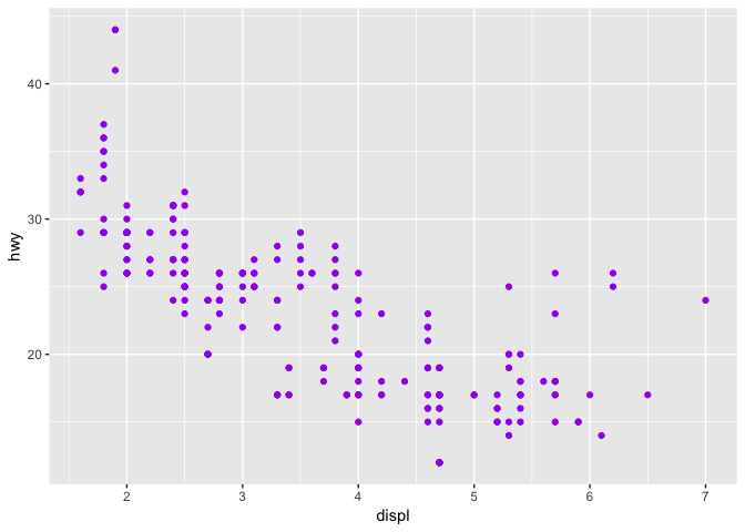

Bean counting

scales 0.5.0.9000-1.0.0.9000: authored 22 PRs, merged 40+ PRs total, 24 contributors to the 1.0.0 release

ggplot2, 3.0.0.9000: opened 18 PRs (2 still open!)

Merged PRs in 3 tidyverse/r-lib packages: scales, ggplot2, and lubridate! Recently vdiffr too!

Intro to Scales: Overview

Scaling 📈

converting data values to perceptual properties.
includes the inverse process: making guides (legends and axes) that can be used to read the graph

Scaling and guides are often some of the most difficult parts of building any visualization.

Scales 📦

The scales package provides the internal scaling infrastructure to ggplot2 and exports standalone, system-agnostic, functions.

Use scales to customize the transformations, breaks, guides and palettes in your visualizations.

Installation

# Scales is installed when you install ggplot2 or the tidyverse.
# But you can install just scales from CRAN:
install.packages("scales")

# Or the development version from Github:
# install.packages("devtools")
devtools::install_github("r-lib/scales")

# let's load it too! Scales is imported by ggplot2 but not loaded explicitly
library(scales)

# For these slides, we'll also want
library(tidyverse)
# for dplyr and ggplot2!

Colour palettes 🎨

scales provides a number of color pallete functions that, given a range of values or the number of colours your want, will return a range of colors by hex code.

# pull a list of colours from any palette
viridis_pal()(4)
#> [1] "#440154FF" "#31688EFF" "#35B779FF" "#FDE725FF"
brewer_pal(type = "div", direction = -1)(4)
#> [1] "#018571" "#80CDC1" "#DFC27D" "#A6611A"
div_gradient_pal()(seq(0, 1, length.out = 4))
#> [1] "#2B6788" "#99A8B4" "#BBA19A" "#90503F"

Color palettes (cont.)

# show_col is a quick way to view palette output
show_col(viridis_pal()(4))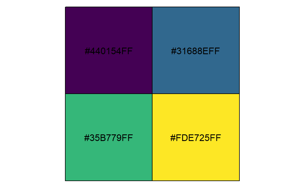

Use scales palettes with baseR

These functions are primarily used under the hood in ggplot2, but can be combined with any plotting system. For example, use them in combination with grDevices::palette(), provided with base R, to affect your base plots…

BaseR example

palette(viridis_pal()(4))
plot(Sepal.Length ~ Sepal.Width, data = iris, col = Species, pch = 20)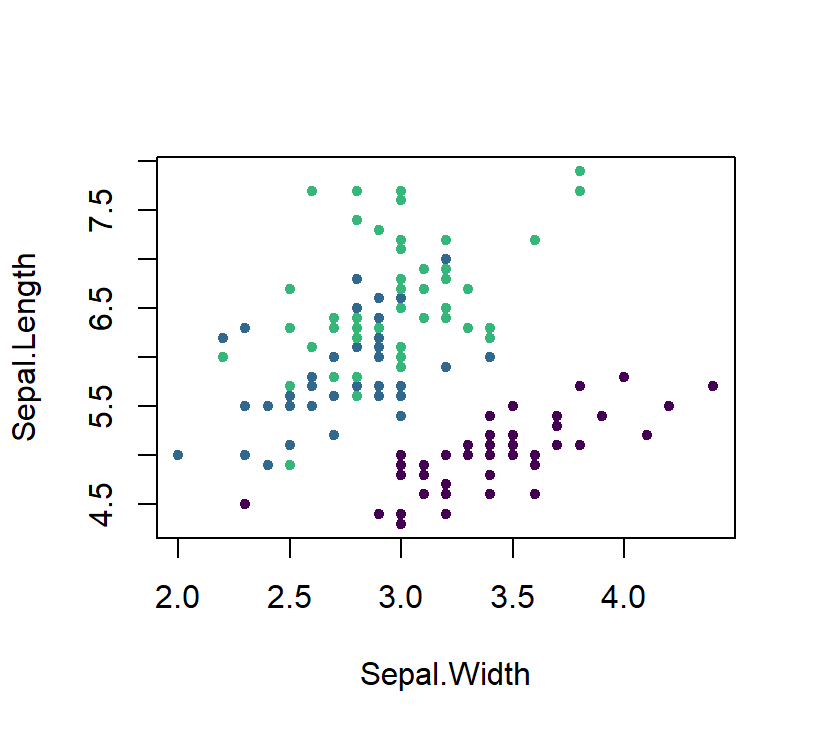

Non-color palettes

Often you want to be able to scale elements other than color. e.g. size, alpha, shape… Of course, scales handles those too!

your_data <- runif(13, 1, 20)
area_pal(range = c(1, 20))(your_data)
#>  [1] 30.37051 79.74341 52.23325 27.88111 81.86193 50.02463 69.63144
#>  [8] 56.08445 67.06121 67.17516 33.24309 81.88239 60.27626
shape_pal()(6)
#> [1] 16 17 15  3  7  8

See these in action in ggplot2

# color examples...
scale_fill_brewer()
scale_color_grey()
scale_color_viridis_c()

# shape examples
scale_shape()
scale_shape_ordinal()

# implement them yourself with...
scale_color_manual()
scale_shape_manual()
scale_size_manual()
# using available scales functions!

Making Guides easy: scales’ formatters

The scales package also provides useful helper functions for formatting numeric data for all types of labels

As of 1.0.0, most of scales formatters are just variations on the generic number() and number_format() functions.

The number formatter

The generic formatter offers consistency in behaviour and arguments across formatters and adds additional functionality for international customization.
With it’s adoption, existing formatters gained new, consistent arguments for scale, accuracy, trim, big.mark, decimal.mark, prefix, suffix etc.

The number formatter, in action

By default, number() will take any numeric vector, round them to nearest whole number, add spaces between every 3 digits and return a character vector useful for feeding to a labels argument in ggplot2.

number(c(12.3, 4, 12345.789, 0.0002))
#> [1] "12"     "4"      "12 346" "0"

Changing defaults

You can easily specify a different rounding behavior, or change the big_mark or decimal_mark for international styling. Even add a prefix or a suffix or scale your numbers on the fly.

number(c(12.3, 4, 12345.789, 0.0002),
  big.mark = ".",
  decimal.mark = ",",
  accuracy = .01
)
#> [1] "12,30"     "4,00"      "12.345,79" "0,00"

Other Formatters:

comma_format() comma() percent_format() percent() unit_format()

date_format() time_format() : Formatted dates and times.

dollar_format() dollar() : Currency formatters, round to nearest cent and display dollar sign.

ordinal_format() ordinal() ordinal_english() ordinal_french() ordinal_spanish(): add ordinal suffixes (-st, -nd, -rd, -th) to numbers.

pvalue_format() pvalue() : p-values formatter

scientific_format() scientific() : Scientific formatter

Examples

# percent() function takes a numeric and does your division and labelling for you
percent(c(0.1, 1 / 3, 0.56))
#> [1] "10.0%" "33.3%" "56.0%"

# comma() adds commas into large numbers for easier readability
comma(10e6)
#> [1] "10,000,000"

# dollar() adds currency symbols
dollar(c(100, 125, 3000))
#> [1] "$100"   "$125"   "$3,000"

# unit_format() adds unique units
# the scale argument allows for simple conversion on the fly
unit_format(unit = "ha", scale = 1e-4)(c(10e6, 10e4, 8e3))
#> [1] "1 000 ha" "10 ha"    "1 ha"

Why the *_format() functions?

Where number() returns a character vector, number_format() and like functions returns a fuctions that can be applied repeatedly or fed to a labels argument in a ggplot2 scale function.

# percent formatting in the French style
french_percent <- percent_format(decimal.mark = ",", suffix = " %")
french_percent(runif(10))
#>  [1] "61,0 %" "32,6 %" "76,0 %" "25,2 %" "51,6 %" "9,9 %"  "14,0 %"
#>  [8] "48,7 %" "98,6 %" "64,9 %"

# currency formatting Euros (and simple conversion!)
usd_to_euro <- dollar_format(prefix = "", suffix = "\u20ac", scale = .86)
usd_to_euro(100)
#> [1] "86€"

Applied in ggplot scales

dsamp <- dplyr::sample_n(diamonds, 1000)
ggplot(dsamp, aes(x = carat, y = price, colour = clarity)) +
  geom_point() + scale_y_continuous(labels = usd_to_euro)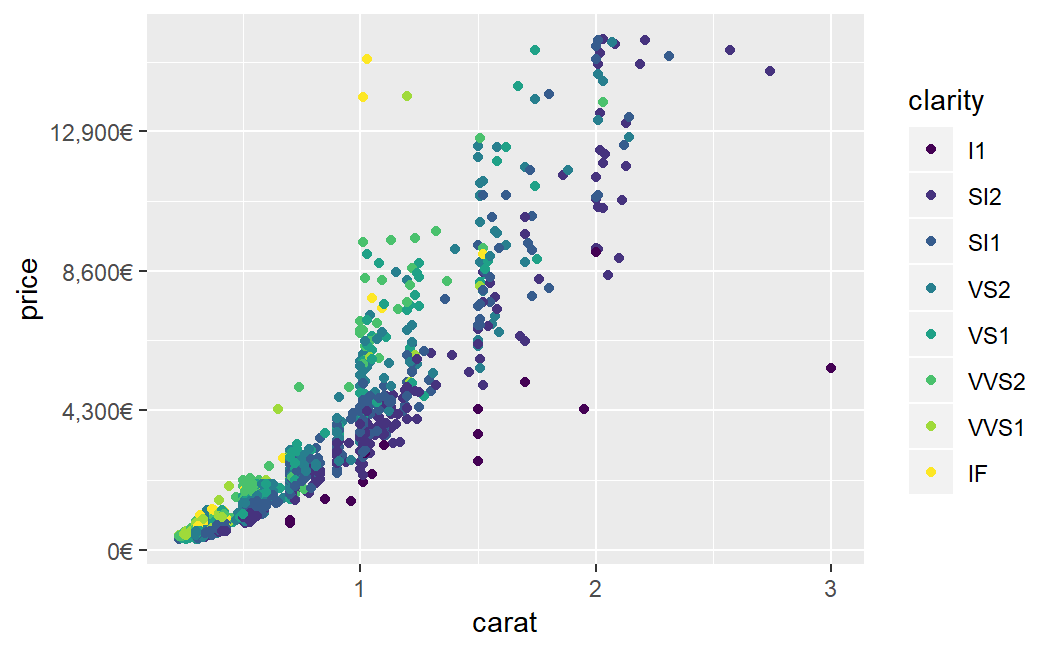

Breaks

scales::extended_breaks() sets most breaks by default in ggplot2

pretty_breaks() is an alternative break calculation

Many of the formatter and transformation functions have matching break functions, eg:

log_breaks() is used to set breaks for log transformed axes with log_trans().
date_breaks() is used to set nice breaks for date and date/time axes.

Bounds & transformations

Rescaling data

scales provides a handful of functions for rescaling data to fit new ranges.

# the rescale functions can rescale continuous vectors to new min, mid, or max values
x <- runif(5, 0, 1)
x
#> [1] 0.4814713 0.2530059 0.7178684 0.8923705 0.9474114

rescale(x, to = c(0, 50))
#> [1] 16.45043  0.00000 33.47198 46.03683 50.00000
rescale_mid(x, mid = .25)
#> [1] 0.6659503 0.5021550 0.8354322 0.9605392 1.0000000
rescale_max(x, to = c(0, 50))
#> [1] 25.40983 13.35248 37.88578 47.09520 50.00000

Squish, Discard, Censor

# squish() will squish your values into a specified range, respecting NAs
squish(c(-1, 0.5, 1, 2, NA), range = c(0, 1))
#> [1] 0.0 0.5 1.0 1.0  NA

# discard will drop data outside a range, respecting NAs
scales::discard(c(-1, 0.5, 1, 2, NA), range = c(0, 1))
#> [1] 0.5 1.0  NA

# censor will return NAs for values outside a range
censor(c(-1, 0.5, 1, 2, NA), range = c(0, 1))
#> [1]  NA 0.5 1.0  NA  NA

Applied to ggplot2

Squish can be really useful for setting the oob argument for a colour scale with reduced limits.

ggplot(iris, aes(x = Sepal.Length, y = Sepal.Width, colour = Sepal.Length)) +
  geom_point() + scale_color_continuous(limit = c(6, 8), oob = scales::squish)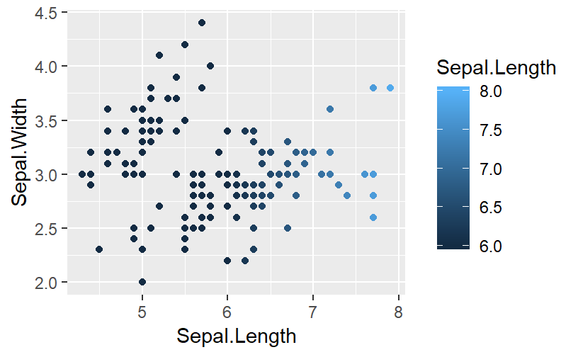

Transformations

scales provides a number of common transformation functions (*_trans()) which specify functions to preform data transformations, format labels, and set correct breaks.

For example: log_trans(), sqrt_trans(), reverse_trans() power the scale_*_log10(), scale_*_sqrt(), scale_*_reverse() functions in ggplot2.

Additional Transformations

asn_trans(): Arc-sin square root transformation.
atanh_trans(): Arc-tangent transformation.
boxcox_trans() modulus_trans() : Box-Cox & modulus transformations.
date_trans() time_trans() hms_trans() : transformations for date, datetime, and hms classes
exp_trans() : Exponential transformation (inverse of log transformation).
pseudolog_trans() : Pseudo-log transformation
probabilty_trans(): Probability transformation

and more…

Building your own transformations

scales also gives users the ability to define and apply their own custom transformation functions for repeated use.

# use trans_new to build a new transformation
dollar_log <- trans_new(
  name = "dollar_log",
  trans = log_trans(base = 10)$trans, # extract a single element from another trans
  inverse = function(x) 10^(x), # or write your own custom functions
  breaks = log_breaks(),
  format = dollar_format()
  )

Applied in ggplot2

# apply our new transformation!
ggplot(dsamp, aes(x = carat, y = price, colour = clarity)) +
  geom_point() + scale_y_continuous(trans = dollar_log)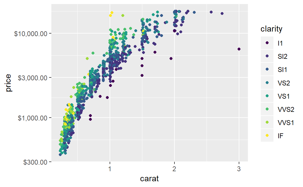

Additional uses

In 1.0.0.9000, scales implements Range() functions to allow users to create their own scales and mutable ranges. These were exported in 1.0.0 but had fatal bugs now fixed in the dev version.

These functions will eventually be imported into ggplot2 to power custom ranges instead of ggproto objects.

Takeaway

scales is a useful package for specifying breaks, labels, palettes, and transformations for your visualizations in ggplot2 and beyond.

Summer Revelations

Open source development is just that open! Open to me AND to you! We need more ladies in dev!

Development work is a wonderful blend of creativity, investigation, puzzle solving, and design. In my view, the pefect hobby and a unique way to give back to the #rstats community.

I want to use my experience in any way I can to help other women get involve in their favorite packages or creating their own!

My Summer @ Rstudio & an intro to the r-lib/scales 📦

My Story 📖

My Summer

Three overarching goals

Prepping scales 1.0.0