Tidy Tuesday is a weekly social data project put on by the R for Data Science Slack learning community (TidyTuesday Repo; R4DS description). The emphasis is on using tidyverse tools to clean and visualize neat data and share it with eachother. I’m not an every week participant but I will share some of my favorite work here and you can see the rest of my visualizations at my github repo linked to this blog post above.
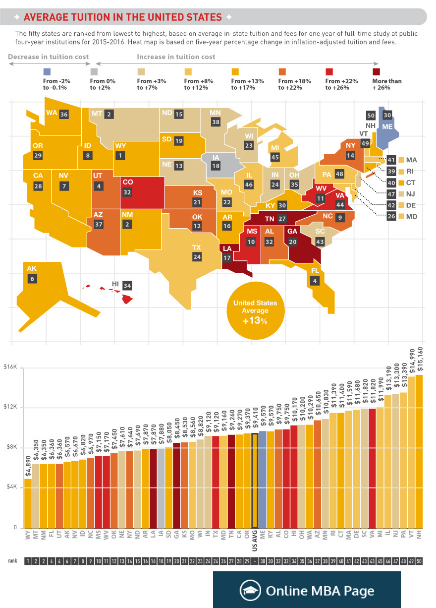
Week 1 deals with US Tuition data and I chose to explore various types of plots
with a focus on the gganimate package. Hope you like it!
Data Sources
Reading in the Data
tuition <- read_xlsx("../data/us_avg_tuition.xlsx")
tuition
## # A tibble: 50 x 13
##    State       `2004-05` `2005-06` `2006-07` `2007-08` `2008-09` `2009-10`
##    <chr>           <dbl>     <dbl>     <dbl>     <dbl>     <dbl>     <dbl>
##  1 Alabama         5683.     5841.     5753.     6008.     6475.     7189.
##  2 Alaska          4328.     4633.     4919.     5070.     5075.     5455.
##  3 Arizona         5138.     5416.     5481.     5682.     6058.     7263.
##  4 Arkansas        5772.     6082.     6232.     6415.     6417.     6627.
##  5 California      5286.     5528.     5335.     5672.     5898.     7259.
##  6 Colorado        4704.     5407.     5596.     6227.     6284.     6948.
##  7 Connecticut     7984.     8249.     8368.     8678.     8721.     9371.
##  8 Delaware        8353.     8611.     8682.     8946.     8995.     9987.
##  9 Florida         3848.     3924.     3888.     3879.     4150.     4783.
## 10 Georgia         4298.     4492.     4584.     4790.     4831.     5550.
## # ... with 40 more rows, and 6 more variables: `2010-11` <dbl>,
## #   `2011-12` <dbl>, `2012-13` <dbl>, `2013-14` <dbl>, `2014-15` <dbl>,
## #   `2015-16` <dbl>
Looking at this I can tell this is going to be ideal for a spatial plot. So I need some US states! Since it’s through time I think I might also try to animate it with gganimate!
# get case to all lower for id to match
data <- tuition %>%
  mutate(id = tolower(State)) %>%
  gather(year, cost, -id, -State)
library(gganimate)
library(fiftystater)

# map_id creates the aesthetic mapping to the state name column in your data
p <- ggplot(data, aes(frame = year, map_id = id)) +
  # map points to the fifty_states shape data
  geom_map(aes(fill = cost), color = "black", map = fifty_states) +
  expand_limits(x = fifty_states$long, y = fifty_states$lat) +
  coord_map() +
  scale_x_continuous(breaks = NULL) +
  scale_y_continuous(breaks = NULL) +
  labs(x = "", y = "") +
  theme(
    legend.position = "bottom",
    panel.background = element_blank(),
    plot.title = element_text(hjust = 0.5, size = 24),
    legend.text = element_text(size = 16),
    legend.title = element_text(size = 16)
  ) +
  guides(fill = guide_legend(title = "Tuition Cost")) +
  ggtitle("US Tuition") +
  scale_fill_gradient(low = "#f7fcf5", high = "#005a32")
p

animation::ani.options(interval = .5)

gganimate(p, ani.width = 1250, ani.height = 585, "tuition.gif", title_frame = TRUE)
What’s going on with Illinois?
Could be cool to plot rate of change instead:
library(lubridate)
##
## Attaching package: 'lubridate'

## The following object is masked from 'package:base':
##
##     date
rates <- data %>%
  mutate(yr_start = mdy(
    paste0("08-01-", str_split(year, "[-]") %>% map_chr(., ~ .[1]))
  )) %>%
  group_by(id) %>%
  mutate(diff_pct = c(0, diff(cost)) / cost)
# map_id creates the aesthetic mapping to the state name column in your data
p2 <- ggplot(rates, aes(frame = year, map_id = id)) +
  # map points to the fifty_states shape data
  geom_map(aes(fill = diff_pct), color = "black", map = fifty_states) +
  expand_limits(x = fifty_states$long, y = fifty_states$lat) +
  coord_map() +
  scale_x_continuous(breaks = NULL) +
  scale_y_continuous(breaks = NULL) +
  labs(x = "", y = "") +
  theme(
    legend.position = "bottom",
    panel.background = element_blank(),
    plot.title = element_text(hjust = 0.5, size = 24),
    legend.text = element_text(size = 16),
    legend.title = element_text(size = 16)
  ) +
  guides(fill = guide_legend(title = "Annual Percent Change")) +
  ggtitle("Annual Percent Change in US Tuition") +
  scale_fill_gradient(
    low = "white", high = "#005a32",
    breaks = c(0, 1, 2, 3, 4, 5, 6, 7, 8, 9, 10)
  )
p2

animation::ani.options(interval = 1)

gganimate(p2, ani.width = 1250, ani.height = 585, "rates.gif", title_frame = TRUE)
A good example where an animation does not make the story clearer!
Let’s play with the geofacet library, see if that can clear things up!
library(geofacet)

ts <- rates %>%
  ungroup() %>%
  select(-id, -diff_pct) %>%
  mutate_if(is.character, as.factor) %>%
  mutate(ease = "linear", year = as.numeric(year(yr_start) - min(year(yr_start)) + 1))

ggplot(ts, aes(year, cost)) +
  geom_line() +
  facet_geo(~ State, grid = "us_state_grid3") +
  scale_x_continuous(breaks = NULL) +
  scale_y_continuous(breaks = NULL) +
  labs(
    title = "Average US State Tuition Costs 2004-2015",
    caption = "Data Source: onlinembapage.com",
    x = "Year",
    y = "Tuition Cost (%)"
  ) +
  theme(strip.text.x = element_text(size = 6), plot.title = element_text(hjust = .5))
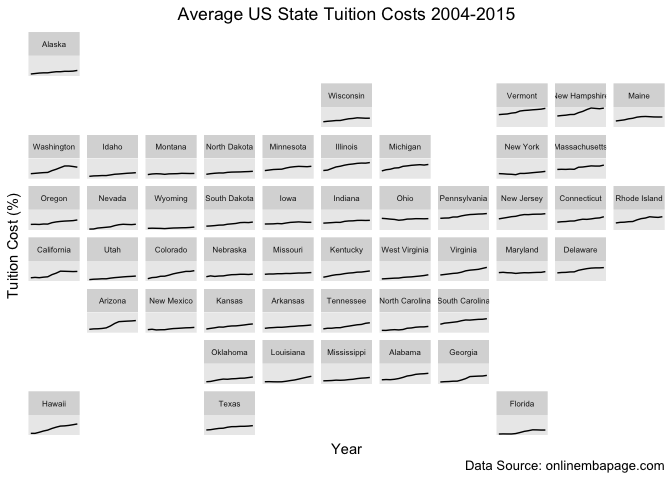
Nice function but the plots are too small for informative axes and the visualization doesn’t quite have the overall punch I would like.
Let’s try making a smooth animated time series plot with a little interpolation help from tweenr!
#### playing with tweenr
## Code adapted from: http://lenkiefer.com/2018/03/18/pipe-tweenr/

library(tweenr)
library(animation)

# filter to just interesting states
ts_fil <- ts %>%
  filter(State %in% c("California", "Vermont", "Illinois", "Wyoming",
                      "Washington", "Florida"))

plot_tween <- tween_elements(ts_fil, time = "year", group = "State",
                             ease = "ease", nframes = 48)
df_tween <- tween_appear(plot_tween, time = "year", nframes = 48)

# add pause at end of animation
df_tween <- df_tween %>% keep_state(20)
summary(df_tween)

make_plot <- function(i) {
  plot_data <-
    df_tween %>%
    filter(.frame == i, .age > -.5)
  p <- plot_data %>%
    ggplot() +
    geom_line(aes(x = yr_start, y = cost, color = .group), size = 1.3) +
    geom_point(
      data = . %>% filter(yr_start == max(yr_start)),
      mapping = aes(x = yr_start, y = cost, color = .group),
      size = 3, stroke = 1.5
    ) +
    geom_point(
      data = . %>% filter(yr_start == max(yr_start)),
      mapping = aes(x = yr_start, y = cost, color = .group), size = 2
    ) +
    geom_text(
      data = . %>% filter(yr_start == max(yr_start)),
      mapping = aes(
        x = yr_start, y = cost, label = .group,
        color = .group
      ), nudge_x = 7, hjust = -0.4, fontface = "bold"
    ) +
    geom_line(data = ts, aes(x = yr_start, y = cost, group = State),
              alpha = 0.25, color = "darkgray") +
    theme_minimal(base_family = "sans") +
    scale_color_manual(values = c("#fec44f", "#253494", "#f46d43",
                                  "#1a9850", "#542788", "#993404")) +
    scale_x_date(
      limits = c(as.Date("2004-08-01"), as.Date("2016-01-01")),
      date_breaks = "1 year", date_labels = "%Y"
    ) +
    theme(
      legend.position = "none",
      plot.title = element_text(face = "bold", size = 24, hjust = .5),
      plot.caption = element_text(hjust = .5, size = 10),
      axis.title.y = element_text(size = 14),
      axis.text.x = element_text(size = 12),
      axis.text.y = element_text(size = 12),
      panel.grid.major.x = element_line(color = "lightgray"),
      panel.grid.minor.x = element_line(color = "lightgray"),
      panel.grid.major.y = element_line(color = "lightgray"),
      panel.grid.minor.y = element_line(color = "lightgray")
    ) +
    labs(
      x = "", y = "Tuition Cost",
      title = "US Tuition by State",
      caption = "Tidy Tuesday Week 1, Data Source: onlinembapage.com, code with considerable help from @lenkiefer's 3/18/18 blog post"
    )
  return(p)
}

oopt <- ani.options(interval = 1 / 10)
saveGIF({
  for (i in 1:max(df_tween$.frame)) {
    g <- make_plot(i)
    print(g)
    print(paste(i, "out of", max(df_tween$.frame)))
    ani.pause()
  }
}, movie.name = "tuition2.gif", ani.width = 700, ani.height = 540)

In order to promote readibility I had to select a subset of states but still pretty cool! Especially given my best attempt to match school colors! Now we can really see tuition is rising steadily! I wonder how it compares to inflation… a visualization for another time perhaps!